Math 1220 Linear Algebra

Subsection 2.5.1 Some matrices whose associated system of equations are easy to solve

The elementary row operations allow us to change matrices and their associated system of linear equations without changing the solutions of those equations. The goal is to end up with matrices which make these common solutions obvious. Here are some examples.

• The augmented matrix

  \begin{equation*} \left[\begin{array}{cccc|c} 1\amp 0\amp 0\amp 0\amp 1\\ 0\amp 1\amp 0\amp 0\amp 2\\ 0\amp 0\amp 1\amp 0\amp 5\\ 0\amp 0\amp 0\amp 1\amp -1 \end{array}\right] \end{equation*}

  corresponds to the system of linear equations

  \begin{equation*} \begin{array}{cccccc} x_1\amp \amp \amp \amp =\amp 1\\ \amp x_2\amp \amp \amp =\amp 2\\ \amp \amp x_3\amp \amp =\amp 5\\ \amp \amp \amp x_4\amp =\amp -1 \end{array} \end{equation*}

  The equations themselves actually describe the unique solution! Notice the structure of the coefficient matrix that makes this possible. There is only one nonzero entry in each row, its value is 1, and as you proceed down through from one row to the next, the nonzero entry moves one column to the right.

• The augmented matrix

  \begin{equation*} \left[\begin{array}{cc|c} 1\amp 1\amp 4\\ 0\amp 2\amp 6 \end{array}\right] \end{equation*}

  corresponds to the system of linear equations

  \begin{equation*} \begin{array}{rcc} x_1+x_2\amp =\amp 4\\ 2x_2\amp =\amp 6 \end{array} \end{equation*}

  The last row is easy to solve: we get \(x_2=3\text{.}\) Using this value, it is also easy to solve \(x_1+x_2=x_1+3=4\text{,}\) or \(x_1=1\text{.}\)

• The augmented matrix

  \begin{equation*} \left[\begin{array}{ccc|c} 1\amp 1\amp 1\amp 4\\ 0\amp 0\amp 2\amp 6 \end{array}\right] \end{equation*}

  corresponds to the system of linear equations

  \begin{equation*} \begin{array}{rcc} x_1+x_2+x_3\amp =\amp 4\\ 2x_3\amp =\amp 6 \end{array} \end{equation*}

  As before, we get \(x_3=3\text{.}\) We still have two variables undefined: we assign a parameter to the second one: \(x_2=t\text{.}\) Using this value, we have \(x_1+x_2+x_3=x_1+t+3=4\text{,}\) or \(x_1=1-t\text{.}\) We now know the solutions: \(x_1=1-t\text{,}\) \(x_2=t\text{,}\) \(x_3=3\) where \(t\) can be any real number. In fact we can check this result with the first equation: \(x_1+x_2+x_3=(1-t) + t + 3=4\text{.}\) The compact way of writing this solution is \((x_1,x_2,x_3)=(1-t,t,3)\text{.}\)

It's clear from the examples given that having lots of zeros in the coefficient matrix is helpful for computing the solutions. It's also clear that if the first nonzero entry in a row is one, then the computation easier. Our plan is to use elementary row operations to change a given coefficient matrix into one with these properties, and then to describe all the solutions. Here are some observations that will help us:

1. If a column has some nonzero entry, we can always make the top entry nonzero by interchanging rows, if necessary using \(R_1\leftrightarrow R_i\) for some \(i>1\text{.}\)

2. If the first nonzero entry of a row \(R_i\) is \(\lambda\text{,}\) we can turn it into a 1 by using \(R_i\leftarrow \tfrac 1\lambda R_i\text{.}\)

3. If two rows \(R_i\) and \(R_j\) have nonzero entries in some column \(k\text{,}\) we can turn the \(j,k\) entry into a zero using \(R_j \leftarrow R_j - \frac{a_{j,k}}{a_{i,k}} R_i\text{.}\)

Subsection 2.5.2 Row echelon form

We now want to define a general class of matrices whose corresponding system of linear equations have solutions that are easy to find. These matrices have a special pattern of zeros and ones, and are said to be in row echelon form.

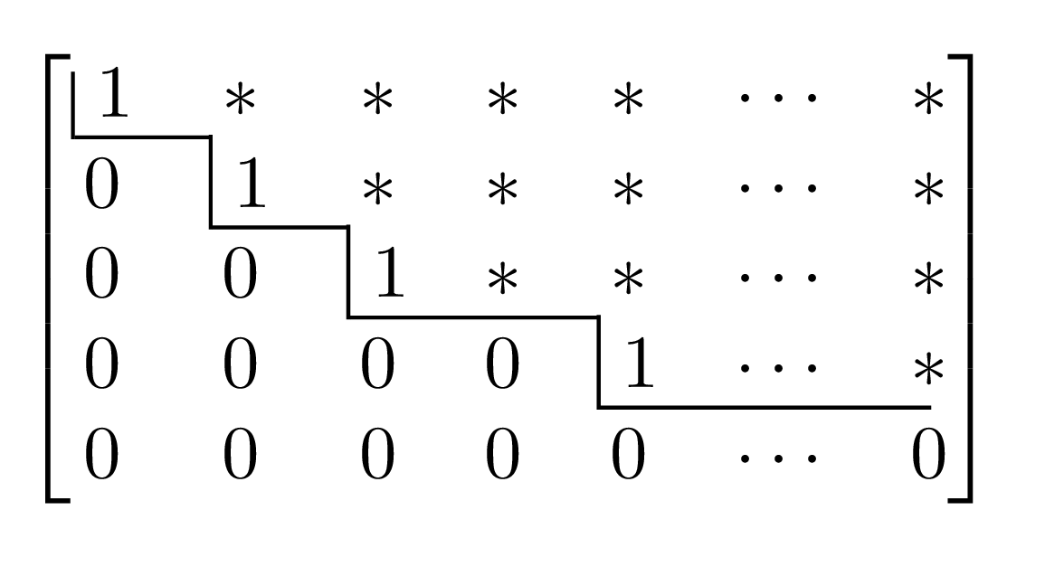
The matrix above gives an idea of what we want. Notice the staircase line drawn through the matrix has all entries below it equal to zero. The entries marked with a \(*\) can take on any value.

The first nonzero entry in a row (if there is one) is called the leading entry. If it equals \(1\text{,}\) then it is called a leading one.

Subsection 2.5.3 The Gaussian elimination algorithm

The plan is now start with the augmented matrix and, by using a sequence of elementary row operations, change it to a new matrix where it is easy to identify the solutions of the associated system of linear equations. Since any elementary row operation leaves the solutions unchanged, the solutions to the final system of linear equations will be identical to the solutions of the original one.

We work on the columns of the matrix from left to right and change the matrix in the following way:

1. Start with the first column. If it has all entries equal to zero, move on to the next column to the right.

2. If the column has nonzero entries, interchange rows, if necessary, to get a nonzero entry on top.

3. Change the top entry, if necessary, to make it a \(1\text{.}\)

4. For any nonzero entry below the top one, use an elementary row operation to change it to zero.

5. Now consider the part of the matrix below the top row and to the right of the column under consideration: if there are no such rows or columns, stop since the procedure is finished.Otherwise, carry out the same procedure on the new matrix.

Here is a first example:

has augmented matrix

We don't need to exchange rows to make the top entry of the first column nonzero, so we proceed to make the top entry \(1\) using the elementary row operation \(R_1\gets \frac13R_1\text{.}\) The matrix becomes

Now we must make all entries below the top one in the column equal to zero. There is, of course, only one such entry, and so, using \(R_2\leftarrow R_2-6R_1\text{,}\) we get

We're now done with the first column, so we continue with the same procedure on the matrix obtained by deleting the first row and first column:

Since there is only one row, we need only change the top entry to \(1\) using division by \(-4\text{,}\) that is, \(R_1\gets -\frac14R_1\text{.}\) We then get

and, putting it back into the original matrix, we get

The matrix is in row echelon form. Now we can determine all of the solutions to the original system of linear equations. The first nonzero entry in the first row is in the first column, the column associated with \(x_1\text{.}\) The first nonzero entry in the second row, similarly, is associated with \(x_2\text{.}\) We assign parameters to the other variables: \(x_3=s\) and \(x_4=t\text{.}\) The second row then tells us that \(x_2-\frac34s =-\frac12 \text{,}\) or \(x_2=\frac34s-\frac12\text{.}\) Now that we know \(x_2\text{,}\) we can use the first row to find \(x_1\text{:}\) we get \(x_1-\frac23x_2-\frac13s+\frac13t=\frac13\text{.}\) We substitute in our known value for \(x_2\) into this equation, and after some simplification, we get \(x_1=\tfrac56s-\tfrac13t\text{.}\) In summary, we have: All solutions to

are of the form

where \(s\) and \(t\) are any real numbers. More compactly, we write this as \((x_1,x_2,x_3,x_4)= \tfrac56s-\tfrac13t,-\tfrac12 +\tfrac34 s,s,t)\text{.}\) In other words, for any assignment of real numbers to \(s\) and \(t\text{,}\) we get a solution to the system of linear equations.

It is easy (and worthwhile) to check that substituting \(x_1,\dots,x_4\) into the two equations does indeed give a solution.

Now consider another example with the equations

and its corresponding augmented matrix as it is changed by Gaussian elimination:

The last row, for any choice of \(x_1, x_2, x_3\text{,}\) reduces to \(0=0,\) so any solution of the associated first three equations will also be a solution to the last one. In other words, the last row of the matrix has no effect on the solution set and may be dropped from the matrix. The third row gives \(x_3=-1.\) The second row gives \(x_2=-1\) and the first row gives \(x_1=-1.\) Hence there is one solution: \((x_1,x_2,x_3)=(-1,-1,-1).\)

Now change the equations from the last example very slightly (the right-hand side of the last equation is changed from \(0\) to \(1\)):

The Gaussian elimination is almost identical as

is reduced to

Now the last row says \(0x_1+0x_2+0x_3=1\text{,}\) which, for any choice of \(x_1\text{,}\) \(x_2\) and \(x_3\text{,}\) reduces to \(0=1\) and is never true. This means the original system of equations have no solutions, that is, the system is inconsistent.

We can make a useful observation here: If a row of the augmented matrix is of the form

where \(*\) is either zero or nonzero, then one of two things happens:

1. \(*=0\) in which case the row may be dropped from the matrix

2. \(*\not=0\) in which case there is no solution.