Math 1220 Linear Algebra

Gauss-Jordan reduction is an extension of the Gaussian elimination algorithm. It produces a matrix, called the reduced row echelon form in the following way: after carrying out Gaussian elimination, continue by changing all nonzero entries above the leading ones to a zero. The resulting matrix looks something like:

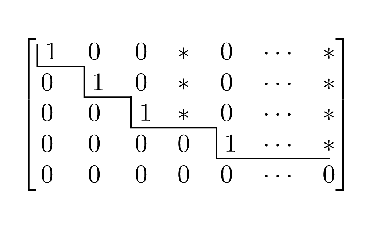
The matrix above gives an idea of what we want. Notice the staircase line drawn through the matrix has all entries below it equal to zero. The entries marked with a \(*\) can take on any value.

For completeness, we'll describe Gauss-Jordan reduction algorithm in detail. As with Gaussian elimination, the columns of the matrix are processed from left to right.

1. Start with the first column. If it has all entries equal to zero, move on to the next column to the right.

2. If, to the contrary, the column has nonzero entries, interchange rows, if necessary, to get a nonzero entry on top.

3. Multiply the top row by a constant to change the nonzero entry to a (leading) one.

4. If there are nonzero entries above or below this (leading) one, use an elementary row operation on each one to change it to a zero.

5. Now consider the part of the matrix below the top row and to the right of the column under consideration: if there are no such rows or columns, stop and the algorithm is finished. Otherwise, carry out the same procedure on the new matrix.

Notice the pattern of zero, 1 and nonzero entries after Gauss-Jordan reduction (with the leading ones in red):

Now that we can put a matrix in reduced row echelon form, let's see what this implies for finding all solutions to the associated system of linear equations. Remember that the first \(n\) columns correspond to coefficients of variables \(x_1,x_2,\dots,x_n\text{,}\) and the last column corresponds to the constants on the right side of the equations. Each column either contains a leading one or it does not. If it does, the corresponding variable is called constrained or basic. If not, the variable is called free. Each free variable is assigned a parameter which may take on any number when finding solutions. The values of the constrained variables are then determined by the reduced row echelon form.

As an example, suppose we have a system of linear equations whose augmented matrix has the following reduced row echelon form:

Notice that this means that our system has three equations and five unknowns. The leading ones are in columns one, three and five, so \(x_1\text{,}\) \(x_3\) and \(x_5\) are constrained variables. This leaves \(x_2\) and \(x_4\) as free variables. We assign parameters to the free variables: \(x_2=s\) and \(x_4=t\text{.}\) The rows of the matrix then determine the constrained variables:

• \(x_5=3\) from the bottom row

• \(x_3 = 2-2t\) from the middle row

• \(x_1=1-2s-t\) from the top row

The compact way of writing this is \((x_1,x_2,x_3,x_4,x_5) = (1-2s-t,s,2-2t,t,3).\)

Notice the role of the zeros above and below each leading one: the evaluation of a constrained variable involves only free variables.

In summary, we can say the following:

1. If the reduced row echelon form has a row of the form \([0,0,\dots,0,1]\text{,}\) then the system of linear equations has no solution.

2. If the reduced row echelon form has no free variables, then it looks like:

   \begin{equation*} \begin{bmatrix} 1 \amp 0 \amp 0 \amp \cdots \amp 0 \amp 0 \amp c_1\\ 0 \amp 1 \amp 0 \amp \cdots \amp 0 \amp 0 \amp c_2\\ 0 \amp 0 \amp 1 \amp \cdots \amp 0 \amp 0 \amp c_3\\ \amp \amp \amp \vdots \\ 0 \amp 0 \amp 0 \amp \cdots \amp 1 \amp 0 \amp c_{n-1}\\ 0 \amp 0 \amp 0 \amp \cdots \amp 0 \amp 1 \amp c_n \end{bmatrix} \end{equation*}

   and there is a unique solution, namely, \(x_1=c_1, x_2=c_2,\dots x_n=c_n\text{.}\)

3. If the reduced row echelon form has free variables, then there are an infinite number of solutions. Indeed, the parameter assigned to any one free variable can take on an infinite number of values.

Consider the following system of linear equations:

The augmented matrix is then put into reduced row echelon form:

Since \(x_3\) and \(x_4\) are free variables, we assign them parameters: \(x_3=s\) and \(x_4=t\text{.}\) We can now evaluate the constrained variables: \(x_1=-1+t\) (from the first row) and \(x_2=2s\) (from the second row). In short, \((x_1,x_2,x_3,x_4)=(-1+t,2s,s,t)\) for any choice of \(s\) or \(t\text{.}\)

Now, as a check, let's put these solutions back into the original equations. \(\begin{array}{rlll} x_1-x_2+2x_3-x_4 \amp =\amp (-1+t) - (2s) + 2(s) - (t) \amp= -1\\ 2x_1+x_2-2x_3-2x_4 \amp =\amp 2(-1+t) + 2s -2s-2t \amp= -2\\ -x_1+2x_2-4x_3+x_4 \amp =\amp -(-1+t) +2(2s) -4s+t \amp= 1 \\ 3x_1-3x_4 \amp =\amp 3(-1+t) -3t \amp= -3 \end{array}\)